Optimization techniques in machine learning.
Introduction
In this article I try to give a quick overview of the optimization techniques in machine learning. This useful mechanics to build a robust, fast and efficient model.
Feature scaling
The name of this normalization method is quite obvious which refers to scale variable to be in the same range. It’s a transformation you need to apply it in your data because some of machine learning algorithm use the magnitude distance between features to work for example k-nearest neighbors (K-NN), Principal Component Analysis (PCA). Also Feature scaling can speed up gradient descent by shorten the step path to converging.
There are two common ways to scale features:
Re-scaling (min-max normalization)
x’ =(x - min(x))/(max(x) - min(x))
Standardization (Z-score Normalization)
x’ = (x - μ)/σ
Batch normalization
The second optimization technique on the table is match normalization. So if feature scaling is a normalization technique for the input layers and the data set features. batch normalization is present to normalize every activation function in the hidden layer. which will be very useful for the gradient descent for better pick of hyper parameter. and helps to avoid the oval shape of GD and transform it to a round shape.

The batch normalization step is hidden after Z computation and the activation computation (there is another method which normalize the activation function).

Implementation:
Mini-batch gradient descent
Mini-batch gradient descent is a variant of gradient descent algorithm has the goal to slice the data set to small “batch” and take benefit of the matrix computation instead of iterate over all. it allow the gradient descent to converge faster in a robust way prevent the whole computation of data set.
If you have an input data ‘X’, Repeat as the number of ‘epochs’ to split it to mini batches, each had the size of ‘mini’. for each batch you need to perform the forward and backward propagation.

RMSProp optimization
Dealing with the gradient descent can be hard to control if the magnitude of the it strongly vary between different weights because the algorithm is just controlling just the sign. RMSProp gives the ability to adapt the step size separately for each weight.

Implementation:
Adam optimization
Adam can be looked at as a combination of RMSprop and Stochastic Gradient Descent with momentum. It uses the squared gradients to scale the learning rate like RMSprop and it takes advantage of momentum by using moving average of the gradient instead of gradient itself like SGD with momentum. Let’s take a closer look at how it works.
Implementation:
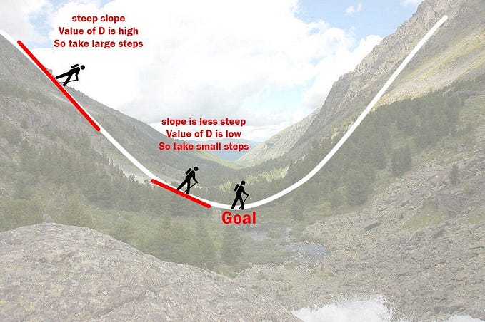
Learning rate decay
The learning rate decay is an optimization methods reduce the learning rate slowly. The gradient descent becomes noisy and never reach the minimum value with constant learning rate. the constant steps continuously overshoot the optimum spot. The learning rate decay reduce the learning rate every time we advance in training depth.